INTRODUCTION
This is an effort to forecast a time series and to create a standard process flow for building an ARIMA model. The sample data looks like,
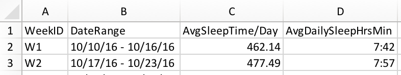
Read the csv data into R and create a time series object using ts() function
sleep<-read.csv("sleep.csv")
sleep.timeseries<-ts(sleep)
head(sleep.timeseries)
## [1] 462.14 477.49 477.79 462.73 439.61 478.56
Plot the timeseries to look for any seasonality or trend in the historical data
plot(sleep.timeseries,xlab = "Week",ylab = "AvgSleepTime/Day")
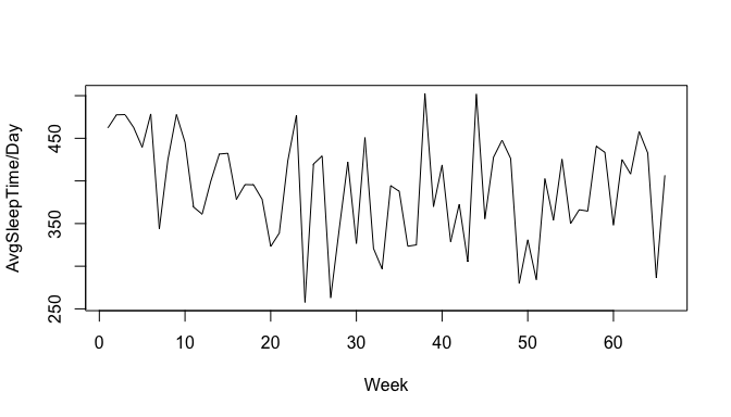
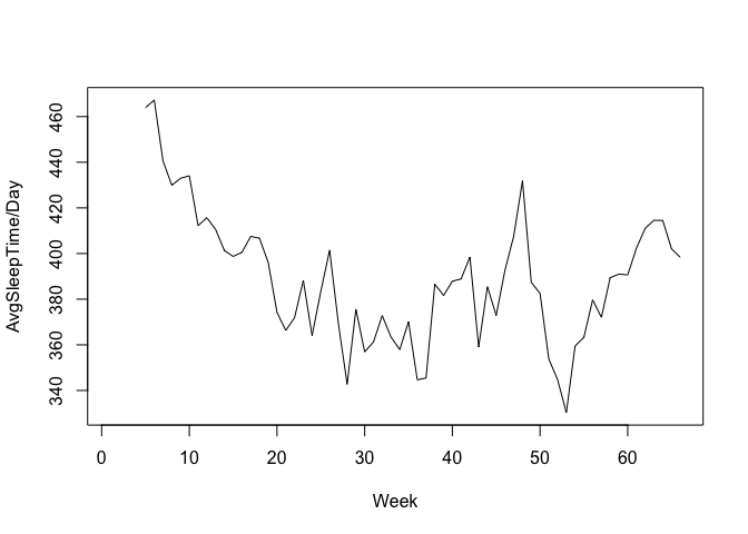
NOTE: Trend - Persistent increase or decrease in the series over a period of time. Seasonality - Recurring regular pattern of up and down fluctuation that occurs each month, each year etc. Based on the inference from above graph, it is clear that there is no seasonal component in the data, though there is a very little downwards trend till week 40(approx) and a gradual upward trend after that. This can be clearly seen, if we try to smoothen the data points using the moving average function SMA() in TTR package. SMA() calculates the arithmetic mean of a series over the past n observations.
library("TTR")
smooth.sleep.timeseries<-SMA(sleep.timeseries,n=5)
plot(smooth.sleep.timeseries,xlab = "Week",ylab = "AvgSleepTime/Day")
ARIMA MODEL
Let us build an ARIMA model to forecast the sleep hours in upcoming days. ARIMA model is defined by 3 parameters as, * AR(Auto Regressive) or p, * I(Integrated) or d, * MA(Moving average) or q And the basic prerequisite for an ARIMA model is that the data should exhibit stationarity.
NOTE: Stationarity - A time series whose mean, variance and autocorrelation structure do not change over time i.e, a flat looking series, without trend, constant variance over time, a constant autocorrelation structure over time and no periodic fluctuations(Seasonality). We need to differentiate the series in order to attain stationarity, as our time series exhibits a trend though it does not have any seasonality.
diff.sleep.timeseries<- diff(sleep.timeseries,differences = 1)
#differences = 1, means first order differentiation
plot(diff.sleep.timeseries,xlab = "Week")
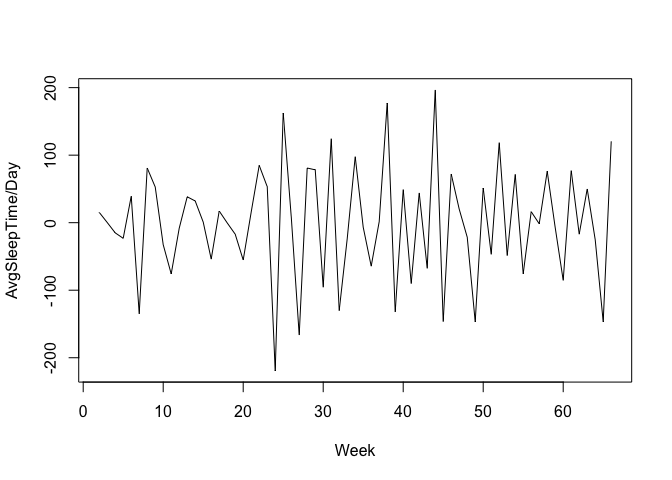
After first order differentiation, the time series looks stationary where its mean, variance doesnot change over time and hence we are good to build an ARIMA model for this series with the parameter d=1. The AR and MA values can be identified based on looking at plots of the autocorrelations and partial autocorrelations. NOTE: Autocorrelation - Autocorrelation of a time series y at lag k is the correlation between y and itself lagged by k periods, i.e., it is the correlation between y t and y t-k. Partial Autocorrelation - The partial autocorrelation of y at lag 2 is the amount of correlation between y t and y t-2 that is not already explained by the fact that y t is correlated with y t-1 and y t-1 is correlated with y t-2. Plot the autocorrelation and partial autocorrelation using acf() and pacf()
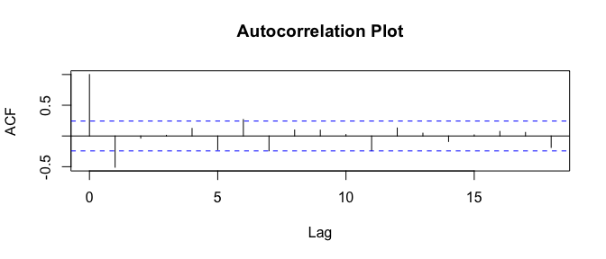
acf(diff.sleep.timeseries,main="Autocorrelation Plot")
pacf(diff.sleep.timeseries,main="Partial Autocorrelation Plot")
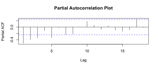
Based on the plots,
- The bar at lag1 on the ACF plot is significant(Spike is taller than the 95% statistically significant band) and negative, followed by a fairly sharp cutoff
- The PACF plot shows a gradual significant decay pattern from below until lag 5
Based on the above observations, we chose either of the below three models, ARMA(p,d,q) We already know d=1, * ARIMA(0,1,1) Significant autocorrelation at lag 1, i.e., “MA(q) signature”, hence choose q=1. This model i.e., MA(moving average) model is usually used to model a time series that shows short-term dependencies between successive observations. * ARMA(5,1,0) Significant Partial autocorrelation until lag 5, i.e., “AR(p) signature”, hence choose p=5. This model i.e., AR(Auto Regressive) model is usually used to model a time series that has its current value, correlated with all the previous ones. * ARMA(5,1,1) Considering both ACF and PACF, choose p=5 and q=1
Let us now fit the first ARIMA model ARIMA(0,1,1),
library(forecast)
sleep.timeseries.arima1<-arima(sleep.timeseries,order = c(0,1,1))
sleep.timeseries.arima1
##
## Call:
## arima(x = sleep.timeseries, order = c(0, 1, 1))
##
## Coefficients:
##           ma1
##       -0.8820
## s.e.   0.0604
##
## sigma^2 estimated as 3691:  log likelihood = -359.93,  aic = 723.86
A residual in forecasting is the difference between an observed value and its forecast based on other observations. To evaluate the ARIMA model, we may follow the below guidlines on its residuals; 1.Residuals should be uncorrelated 2.Residuals should have zero mean 3.Residuals should have constant variance 4.Reiduals should be normally distributed
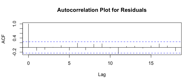
Plot an autocorrelation to conclude residuals are not correlated, if all the spikes are within the statistically significant 95% band.
acf(sleep.timeseries.arima1$residuals,main="Autocorrelation Plot for Residuals")
Check the mean for residuals using mean() function
mean(sleep.timeseries.arima1$residuals)
## [1] -8.589026
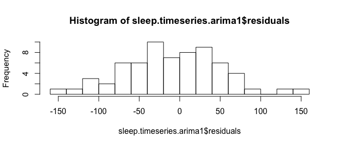
Plot a histogram to check whether the residuals are normally distributed and have zero mean and constant variance.
hist(sleep.timeseries.arima1$residuals,breaks=IQR(sleep.timeseries.arima1$residuals/4))
To further test the autocorrelation, we can perform Ljung-Box test using Box.test(), where the resulting p value can be interpreted in the following ways, If p-value < 0.051: Values are showing dependence on each other i.e. possibility of correlation If p-value > 0.051: Dependance of values cant be confirmed
Box.test(sleep.timeseries.arima1$residuals,lag=20,type = "Ljung-Box")
##
##  Box-Ljung test
##
## data:  sleep.timeseries.arima1$residuals
## X-squared = 21.742, df = 20, p-value = 0.3547
Based on the above tests, We could infer that the mean is non-zero and negative though the variance is uniform and there is no significant autocorrelation found. We can iterate the same test process for the next model and validate its fit or we can use auto.arima() function to choose a better model.
auto.arima(sleep.timeseries)
## Series: sleep.timeseries
## ARIMA(0,1,1)
##
## Coefficients:
##           ma1
##       -0.8820
## s.e.   0.0604
##
## sigma^2 estimated as 3749:  log likelihood=-359.93
## AIC=723.86   AICc=724.05   BIC=728.21
Based on the above tests and also as auto.arima() function has suggested, ARIMA(0,1,1) model is fixed for forecasting the future sleep hours value.
forecast() function is used and the parameter ‘h’ represents the number of future value we would like to forecast.
Let us choose h=1, which represents that we would like to forecast the average sleep hours per day for next one week.
forecast.sleep.timeseries.arima1<-forecast(sleep.timeseries.arima1,h=1)
forecast.sleep.timeseries.arima1
##    Point Forecast    Lo 80    Hi 80    Lo 95    Hi 95
## 67       389.8374 311.9759 467.6989 270.7585 508.9163
plot(forecast.sleep.timeseries.arima1)
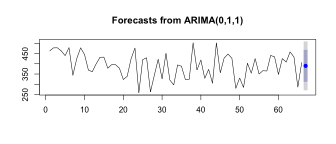
Comparison between different ARIMA model forecast results ARIMA(0,1,1)
##    Point Forecast    Lo 80    Hi 80    Lo 95    Hi 95
## 67       389.8374 311.9759 467.6989 270.7585 508.9163
ARIMA(5,1,0)
##    Point Forecast    Lo 80    Hi 80   Lo 95    Hi 95
## 67       423.6551 347.8669 499.4433 307.747 539.5632
ARIMA(5,1,1)
##    Point Forecast    Lo 80    Hi 80    Lo 95    Hi 95
## 67       414.0314 338.9802 489.0826 299.2505 528.8124
ARIMA(5,2,1)
##    Point Forecast    Lo 80    Hi 80    Lo 95    Hi 95
## 67       420.6297 343.6835 497.5759 302.9506 538.3087
Conclusion
A basic time series forecasting process has been used to forecast and based on the ARIMA(0,1,1) model, the forecast is 389.83
References
- Using R for Time Series Analysis by Avril Coghlan
- Notes on nonseasonal ARIMA models by Robert Nau